Advent of Code 2024: Summary of Days 7 to 12

This page serves as the second part of a summary of my experience with Advent of Code 2024, covering days 7 to 12. For the first 6 days see my previous post.

As mentioned previously and in the Advent of Code FAQ, I will avoid including the full puzzle text or raw inputs in this post, and I’ll be referring to each part of the question as Part A and Part B.

Day 7

Starting of the Saturday, Day 7 was on par in difficulty with the previous days. It involved discovering which operators would result in a given value and adding them together.

My approach to Part A of this question involved creating a Python enum to hold the possible operators and implement them in a single place. The first 2 operators, addition and multiplication, were trivial to implement. Python’s excellent standard library made it relatively easy to generate the possible operators for each line of input using itertools.product.

Part B added a single new operator, concatenation. Again the flexibility of Python meant I could add this a simple operation using strings int(f"{a}{b})". Of course, this is likely slower than doing the equivalent math. I will revisit this to optimise it further.

Day 8

Day 8 came out on a Sunday. Unfortunately, I was very busy that day so I only managed to look at the problem in earnest in the evening. With my tired eyes I still managed to complete Part A, but the wording on both questions proved a little difficult to decipher at the time.

Again, itertools really helped with these challenges. This time it was the combinations function that proved useful in getting the unique combinations of antennas.

Part A was relatively simple once you understand the problem. Simply find the difference between the two antennas points and project a point from each in either direction. I struggled to get the correct answer to this briefly, as I made a mistake when loading the puzzle input and increased the width of my grid by a single digit! This didn’t break the example given, but with the actual puzzle input I had it resulted in 14 extra antinodes appearing along the rightmost column.

After some well earned rest, I was able to tackle Part B. This just consisted of creating antinodes at every interval along the lines produced by two antennas. This interval is the distance between the two antennas.

Day 9

So Day 9 seemed like a spike in difficulty compared to the previous days. These challenges invoked memories of running disk defragmentation software in the early 2000s.

For both parts, you take the puzzle input and decode it to represent a disk containing files and free space, and then operate on it:

Then the objective of Part A was to move blocks of data so they are all next to each other, before finally calculating a simple checksum.

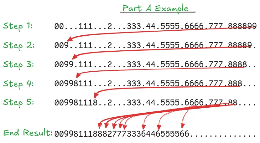
Initially, my solution to Part A involved me converting the input string into an expanded string, similar to how the examples were explained in the question. This worked well for the example input, as it only included 10 total unique IDs, but when ran on the real puzzle input my code was faulty.

Eventually, after much time spent frustrated, I looked to the internet for some hints, careful to avoid any full solutions. It didn’t take long to see that others had made a similar mistake. In the actual puzzle input there are many more unique IDs than the 10 in the example. As a consequence of using a string the IDs that are greater than 9 were being treated as multiple IDs between 0-9.

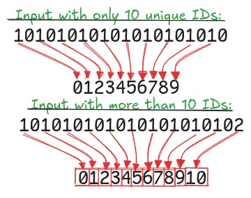
Thankfully, with the problem known, it was simple to rectify, instead of creating a new expanded string I instead stuck with a list of either IDs or None entries like so list[Optional[int]].

As anyone who ran disk defragmentation in the past knows, storing all your data close together is all well and good, but what you really want is like for like data near each other so you avoid those time consuming seeks. This was the objective of Part B. I solved this by using a simple algorithm that walked from the end of the list backward, then when it found a chunk of non-empty data I would pause and then search from the front of the list for an empty space large enough for that chunk and move it there. After which the backward search would continue.

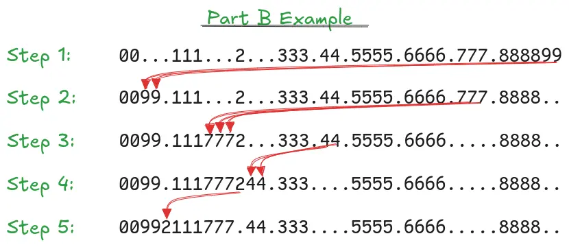
This algorithm is relatively slow as it will search for empty space for every block of non-empty data found. I could improve upon this by keeping track of both what data was moved and an index of the empty space available. I may revisit this, time permitting.

Day 10

Day 10 assigns us challenges involving a topographic map. Thankfully, the inputs use only the numbers 0-9 to represent various heights. These can be mapped easily to greyscale.

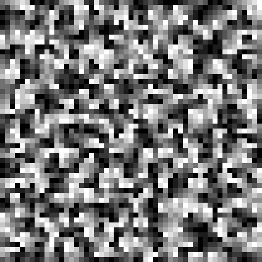
Part A requires us to find trailheads and add up their scores. A trailhead is made from paths on the map. These paths have to start at a value of 0 and end on a value of 9, with each step only increasing the tile value by 1. In this challenge we can only move in the cardinal compass directions, i.e. North, East, South, or West. The trailhead score is the count of 9 height tiles reachable from its 0 height start.

You can solve Part A with a modified flood-fill algorithm. Starting at a 0 height, at each stage you’d be looking for values that are 1 higher up until 9. Scoring becomes a matter of counting the unique 9-height tiles reached.

Being familiar with pathfinding problems, I noticed you can potentially do some optimisations to reduce the search space, these were ultimately unneeded as using the contents of the flood-fill is enough to limit calculations in both parts.

One optimisation that can be done is in finding the trailheads: You can find all the starts and ends of possible trails by simply searching for 0 and 9 height tiles on the map, then with these positions, you can create pairs of potential trail starts and trail ends. Because we can only move 1 value up in height at a time, we know that any ending points that are further away than 9 steps (0 to 9) cannot possibly be reached. We can even avoid using the proper 2D distance formula to measure this distance because we cannot travel diagonally.

Below is an example of these kind of distance functions:

from math import sqrt
from typing import TypeAlias

XY: TypeAlias = (int, int)

# This is the 2D distance formula
def dist(a: XY, b: XY) -> float:
    return sqrt(pow(b[0] - a[0], 2) + pow(b[1] - a[1], 2))

# This is an approximation we can use
# Since we cannot move diagonally, simple addition works
def taxicab_dist(a: XY, b: XY) -> int:
    return abs(b[0] - a[0]) + abs(b[1] - a[1])

# In theory taxicab_dist will be faster as it doesn't do a square root
# In practice the difference may well be negligible as modern CPUs 
# have dedicated instructions for square root

As you can see from the examples below the min “taxicab” distance an end tile can be from a start tile is 1 and the maximum is 9:

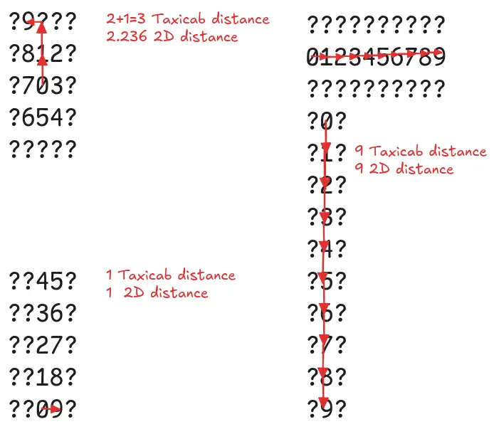
So a modified flood-fill solves Part A, but Part B requires you to keep track of unique paths, which means each start and end pair can have multiple paths. Thankfully, our flood-fill from Part A can serve as a way of limiting any more advanced search.

If we modify our flood filling algorithm to make a note of all the possible sources a tile can be reach from we end up building a graph.

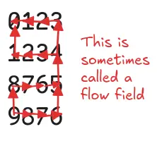
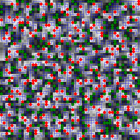
From this graph, sometimes called a flow field, we can easily generate all the possible unique paths, solving Part B. Below is a visualisation of all these paths on my input:

Day 11

Day 11 takes us back to a set of 1 dimensional challenges involving an ever growing list. Part A introduces us to our problem space, a list where the contents change after each “blink” based on some rules. This is very much reminiscent of a Cellular Automaton although in a single dimension rather than 2.

Part A was very simple, naively applying the rules to the input works in a quick amount of time. Part B however, asks you to run the rules for much longer, and applying the rules naively will quickly run you out of memory and take an inordinate amount of time.

So how do we solve Part B?

One thing we can do is examine the rules for any ways we can optimise their application.

• If the stone is engraved with the number 0, it is replaced by a stone engraved with the number 1.
• If the stone is engraved with a number that has an even number of digits, it is replaced by two stones. The left half of the digits are engraved on the new left stone, and the right half of the digits are engraved on the new right stone. (The new numbers don’t keep extra leading zeroes: 1000 would become stones 10 and 0.)
• If none of the other rules apply, the stone is replaced by a new stone; the old stone’s number multiplied by 2024 is engraved on the new stone.

Even without diagramming the rules it seem obvious that there exist some patterns:

• 0 is always turned to a 1 which will then turn into a 2024 on the next iteration
• The number of stones will always increase due to the turning of 0 to 1 to 2024
• Numbers will inevitably tend towards multiples of 2024 due to the third rule
• As soon as we get a number with an even count of digits we will inevitably reach single digits as we apply the rules, which will again tend towards multiplying by 2024

So I decide to analyse the pattern the rules produce for a single input of 0. I did this by hand and produced this monstrosity:

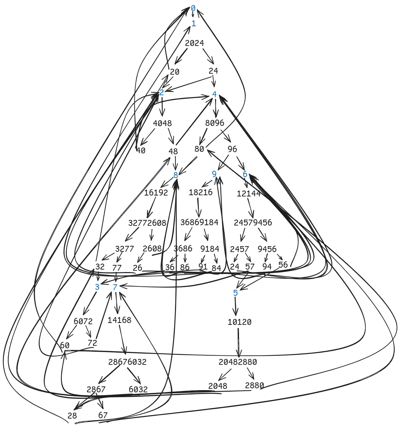
While it may be hard to see, I have highlighted all the single digits in blue.

I am sure you can write code to use this kind of tree-like structure, but that would be time consuming and difficult. So I opted for another approach, Memoization.

I essentially kept a cheat sheet of number and iteration to the count of results. Then when I run my code on each single element in the given input I can reuse these results and severely reduce the computation.

If coded recursively, a single call to solve(stone=0, iterations=75) will populate the cheat sheet with all the values in the above tree, and reuse them when needed. Then subsequent runs for other numbers help populate this cheat sheet more and more.

Day 12

Day 12 returned to a set of 2 dimensional map puzzles. This time they focus on extracting regions from a map, finding their perimeter and areas.

Part A was very simple. In fact, I again used a flood-fill algorithm to find all the regions in the input. For perimeter I simply scanned each regions contents for tiles that were not fully surrounded by members of the same region. I could have done this when initially building the region to speed up this part, however it was conceptually easier to do this after building the regions.

Part B was again a nice little increase in difficulty. Instead of calculating total perimeter, you needed to find the sides of the regions. This is still relatively simple since you have the regions from part A.

Overall

This was the second post detailing 6 days of Advent of Code 2024. If you want to view my post on days 1 to 6 you can do so here.

Overall, the challenge has increased from the first 6 days, with at least one puzzle, Day 11, not being amenable to a brute force approach.

I am enjoying these days so far, and I think this is the furthest I have got with Advent of Code in some years! I especially enjoyed Days 9 and 10, along with Part B of Day 11, which I puzzled over the course of a day.

I’d love to hear how you are finding it, and also please share any links to interesting breakdowns of the problems by others. I’m already following Josiah Winslow’s posts with interest, and even simplified my solution to Day 12 Part B based on his example.